A storage benchmark becomes interesting when the fastest number is not its main result. MLPerf Storage 2.0 reported more than 200 performance results from 26 organizations in August 2025[1]. The submissions covered local drives, shared filesystems, block and object storage, software-defined systems and in-storage acceleration. That breadth makes a single winner meaningless. What the suite offers instead is a controlled way to ask two operational questions: how many accelerators can this system keep busy, and how quickly can a failed training job save or recover its state?
Those questions are more useful than a sequential-bandwidth specification. Training reads many records through framework data loaders while thousands of workers advance together. Checkpointing reverses the direction and makes every rank write state at nearly the same time. A system can look strong on one path and weak on the other. Version 2.0 therefore separates training from checkpointing and publishes the configuration, logs and system description behind each result[2].
The benchmark uses simulated GPUs on purpose
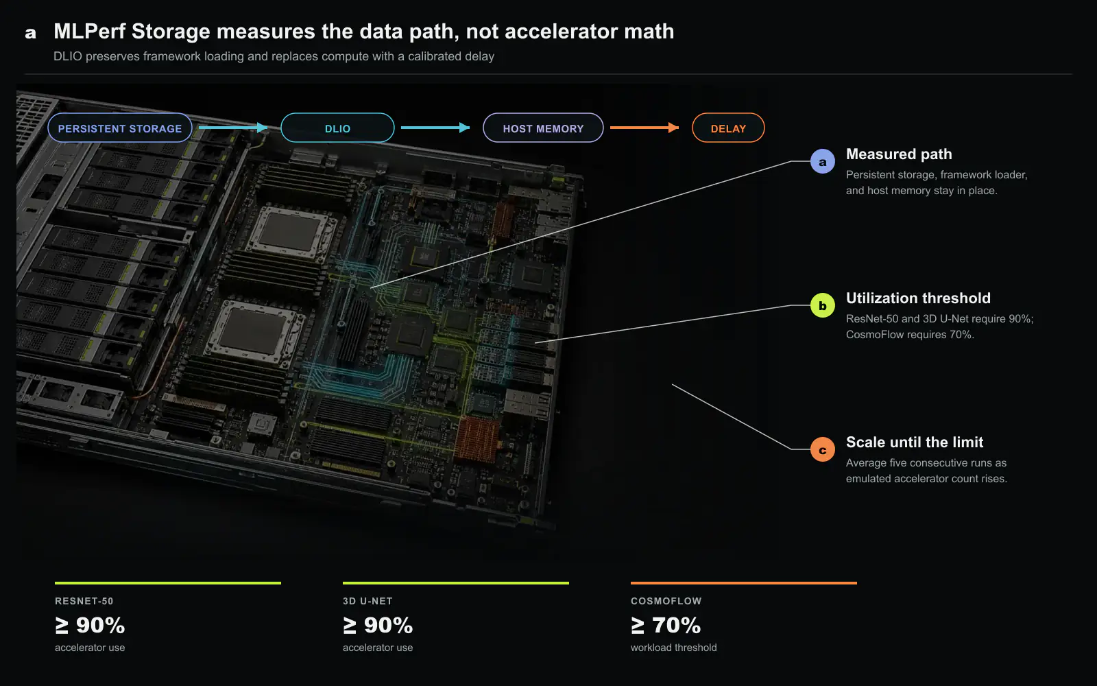
The training test does not require the submitter to own the GPUs named in a result. DLIO, a tool developed at Argonne National Laboratory, runs the real framework-side data path and replaces accelerator computation for each batch with a measured delay. Storage still supplies files through PyTorch or TensorFlow into host memory, while a sleep() represents the time that an A100 or H100 would have spent computing. Transfers from host memory into accelerator memory are outside the measured path.
This design makes scale a variable rather than a capital purchase. A submitter increases the number of emulated accelerators until I/O can no longer sustain the target utilization. Five consecutive runs are required, and the final metric is their average. Failed runs cannot be removed from the middle of a selected sequence. Thus, the reported accelerator count describes a sustained operating point, not a one-off burst.
The three workloads also have different pass lines. ResNet-50 uses small ImageNet-like records and requires at least 90% accelerator utilization. 3D U-Net reads much larger medical-imaging samples and has the same 90% threshold. CosmoFlow targets 70%, reflecting its own compute and I/O profile[2]. Treating every row as if 90% applied would incorrectly reject valid CosmoFlow submissions.
Scale and bandwidth answer different questions
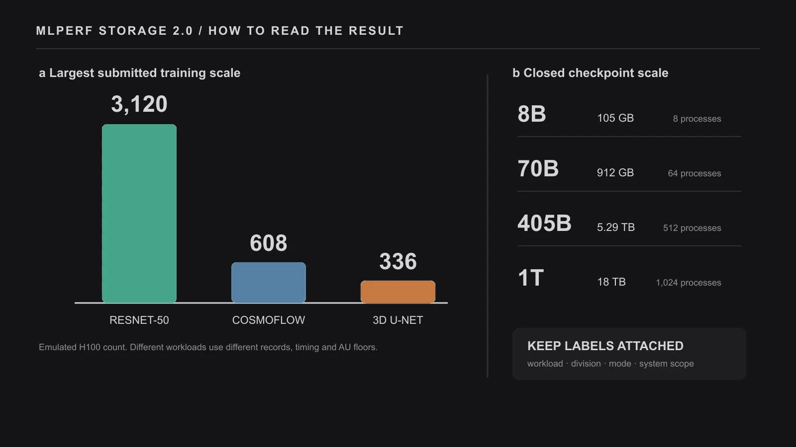
The published CSV files show why both axes matter[3]. Among the submitted training configurations, the largest reported scales reached 3,120 emulated H100s for ResNet-50, 608 for CosmoFlow and 336 for 3D U-Net. The highest observed mean I/O rates did not occur at all three maximum-scale points. They were approximately 384 GB/s for ResNet-50 at 2,160 emulated H100s, 280 GB/s for CosmoFlow at 528 and 490 GB/s for 3D U-Net at 176.
These numbers are not a three-row product ranking. Record sizes, batches, computation delays and utilization thresholds differ by workload. Even within one workload, the largest accelerator count and the largest measured bandwidth can belong to different runs. Scale asks how far a configuration remains above its utilization floor. Bandwidth describes the volume moved at a particular point on that curve. Procurement needs both.
Version 2.0 also preserves comparability with version 1.0 for the three training workloads. MLCommons says participating systems supported roughly twice as many accelerators as in the earlier round[1]. That statement is a suite-level observation, not proof that every storage architecture doubled. Software versions, client counts, network topology and submitted system sizes still need to be read from each disclosure.
A trillion-parameter checkpoint is a synchronized event
The new checkpoint track models four Llama scales: 8B, 70B, 405B and 1T. The 8B, 70B and 405B full states are listed as 105 GB, 912 GB and 5.29 TB. For 1T, the public materials need a version label: the launch explainer says 15 TB, including 13.2 TB of optimizer state, while the current rules table says 18 TB[2][4]. Closed-division runs fix the process counts at 8, 64, 512 and 1,024. A default run writes and reads the complete distributed checkpoint. A separate subset mode lets one host exercise its local share, but subset and full results must not be compared as if they moved the same data.
Each submission writes ten checkpoints, clears filesystem caches when required, then reads ten checkpoints. fsync is enabled so that a completed write reaches stable storage. For every run, duration is the slowest process and throughput is the slowest process’s rate. This conservative reduction matters because a distributed job can resume only after its last rank is ready.
The full-scale results demonstrate the size of the event. One closed 405B submission wrote its 5.29 TB checkpoint in a mean 5.69 seconds, reported as 930.2 GB/s. Another recovered the same model scale in 8.01 seconds, or 660.9 GB/s. At 1T, one closed result reports 34.82 seconds for writing at 444.6 GB/s and 22.29 seconds for reading at 692.4 GB/s. Its CSV stores 15,426.6 under checkpoint_size_GB. That field is the right denominator for reproducing the submitted throughput; “15 TB” and “18 TB” are labels in different official documents, not permission to substitute one nominal size into the calculation. This documentation drift is precisely why benchmark rows should travel with their versioned rules and raw result files.
Four labels must stay attached to every number
The suite becomes misleading when a result loses its workload, division, mode or system scope. Open submissions may alter the prescribed configuration if they disclose the change. Closed submissions restrict those changes for comparability. A local subset checkpoint measures one node’s assigned shards, whereas a default checkpoint includes the whole distributed state. Client nodes and network links are also part of the submitted system, so a storage-array name alone does not reproduce a result.
Caching deserves the same care. The rules require caches to be cleared when the checkpoint share per client is small enough to remain resident in memory. Any remapping step needed before another host can read a checkpoint must be timed and added to recovery. These provisions keep “saved” and “recoverable elsewhere” from becoming two different claims.
There are still important omissions. Training computation is modeled rather than executed, host-to-device transfer is excluded, and version 2.0 does not benchmark online or offline preprocessing. It does not reproduce application-level burst alignment, metadata behavior or failure patterns in every real cluster. The result is therefore not a purchase order. It is a repeatable stress curve that tells an operator where to perform the next, application-specific test.
Checkpoint bandwidth is reliability capacity
Storage procurement often treats training I/O and checkpointing as two throughput tests. At cluster scale they are different economic functions. Training I/O determines whether accelerators receive data fast enough during normal operation. Checkpointing determines how much work the system can afford to lose when failures become frequent. A faster checkpoint path can justify a shorter interval, reduce rollback, and return a recovered job sooner. Its value rises with cluster size even if the input dataset and per-GPU data rate remain unchanged.
This is why a peak GB/s result cannot be converted directly into supported GPU count. The decision needs checkpoint size, coordinated write duration, restore duration, failure interval, framework pause behavior, and the utilization threshold used by the simulated accelerators. Tail time matters because the slowest rank or storage target can hold the whole job at the barrier. A system with a lower peak but tighter completion distribution may protect more training progress than one with a higher aggregate number and a long tail.
An acceptance test should connect the two MLPerf modes into one useful-accelerator-time metric. Measure normal training utilization, initiate checkpoints at realistic intervals, inject a failure, restore the latest state, and report the accelerator time that contributes to work over the entire cycle. Repeat under metadata pressure and concurrent jobs, since an isolated benchmark does not price interference in a shared neocloud. MLPerf Storage 2.0 supplies a reproducible method for comparing the components. The buyer still has to assemble them into the metric that matters: the fraction of rented accelerator time that survives both data delivery and recovery.
A benchmark result is a configuration, not a product label
MLPerf Storage creates a common workload, but every result still belongs to a specific client count, model, checkpoint pattern, file-system or object configuration, network, capacity, cache state, and software version. Removing any of those labels turns a reproducible measurement into a marketing number. Buyers should compare entries only after deciding which dimensions match their intended workload.
The simulated GPU method is a strength because it isolates storage and reaches scales that a test lab may not equip with accelerators. It also means the client system must reproduce the timing and concurrency of the target training workload. If CPU, memory, or network limits the simulators, the result measures the load generator. Submissions should therefore include client resource use and evidence that requested I/O was issued on schedule.
Cache state deserves explicit treatment. A warm metadata or data cache can represent repeated epochs or a tuned production path, while a cold run can represent restart or first use. Neither is universally correct. The result should state which state was measured and, where possible, show both so an operator can see how much performance depends on retained cache.
Translate the score into a checkpoint deadline
Peak bandwidth is useful only after it is connected to the amount of state and the time available to protect it. A training team should begin with checkpoint bytes, frequency, number of writers, acceptable pause, and the recovery-point objective. Dividing bytes by the deadline gives a minimum sustained rate, but metadata, synchronization, replication, and tail behavior add margin.
The system should then be tested at that deadline while normal training I/O and network communication continue. A checkpoint path that reaches its score in isolation may contend with data loading or collectives in production. The important outcome is whether every writer completes and the checkpoint becomes recoverable before the next protection point, not whether aggregate counters briefly cross a target.
Frequency creates a second trade. Faster checkpoints can reduce the interval between them and lower lost work after failure. More frequent checkpoints also consume more background bandwidth and capacity. The optimal point depends on failure rate, checkpoint time, restart time, and storage cost. Reporting those inputs turns a storage result into a reliability decision.
Scaling must preserve failure and rebuild behavior
A system can scale bandwidth by adding storage nodes while making each checkpoint depend on more components. The benchmark should be paired with node and path failure tests, degraded-mode throughput, and rebuild impact. If one failed node cuts bandwidth below the checkpoint deadline for hours, the nominal scale result overstates deliverable protection.
Capacity growth also changes metadata and namespace pressure. A trillion-parameter checkpoint contains large objects, but training and data pipelines may create many smaller files around it. Client startup, directory operations, deletion, and retention policy can become bottlenecks outside the measured bulk path. Production qualification should include the complete checkpoint lifecycle and concurrent datasets.
Network topology must remain attached to client count. Adding simulated GPUs across more racks can increase bisection demand and expose oversubscription that a smaller run did not see. Conversely, concentrating clients can bottleneck a few host links. The report should map clients and storage endpoints to racks and show where traffic crosses tiers.
Procurement should use two matched replays
The first replay follows the standard benchmark exactly and establishes comparability. The second uses the buyer’s checkpoint size, writer count, burst timing, dataset traffic, and failure conditions. A system that performs well on both offers evidence that the standard score transfers. A gap between them is not necessarily a failure, but it identifies which workload feature the contract must address.
Cost should be divided by successful protected work. Include storage nodes, client and network equipment, software licenses, usable capacity after replication, power, and operational reserve. Then normalize by checkpoint bytes committed within the deadline or by accelerator-hours protected. This prevents a design from appearing cheaper because it omits redundancy or misses the time window that gives the checkpoint value.
We read MLPerf Storage 2.0 as a disciplined starting point for this process. It makes scale and workload conditions more comparable and demonstrates that accelerator fleets can be emulated for storage testing. The result becomes a purchasing claim only when configuration labels, cache state, checkpoint deadline, degraded operation, and the buyer’s own replay remain attached.
Source and attribution
This article is an editorial analysis prepared by Silicon & Systems from the MLPerf Storage 2.0 rules, checkpoint explainer, announcement and public result files. All explanations and figures were created for this article; no source table or figure is reproduced. MLPerf is a trademark of MLCommons. The benchmark code and result repository are distributed under the Apache License 2.0, while the official results announcement provides the release context. Vendor-written supplemental descriptions were treated as disclosures, not independent evaluations.