Datacenter SSD prediction is an imbalanced decision problem. Healthy drives produce millions of daily telemetry samples; failed drives are rare. A classifier can achieve high accuracy by predicting health almost everywhere, yet miss the events operators care about. Conversely, a sensitive detector can generate enough false replacements to erase its reliability value.
Downsampling healthy data balances training, but random removal discards exactly the healthy samples most useful for defining a failure boundary. Feature selection creates another loss. A telemetry attribute weak by itself may become decisive when paired with an error count or a change rate. A global importance score does not reveal that conditional range to an operator.
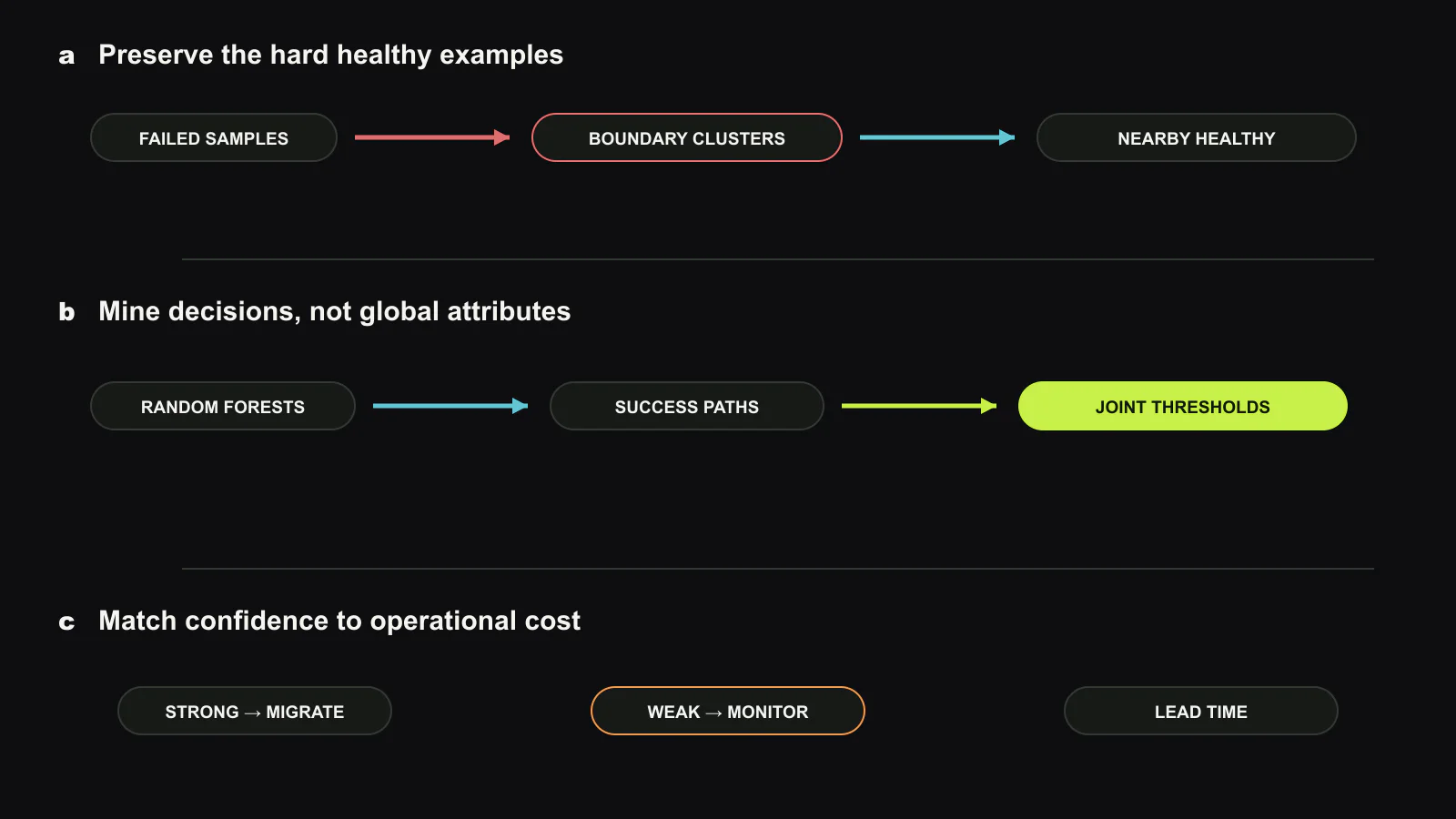
FailureMiner preserves near-boundary examples and interprets decisions rather than attributes. It trains random forests, identifies branches that correctly reach failed drives, assigns contribution to threshold decisions, and mines combinations that recur together. The output is a small set of human-readable rules such as an increase in uncorrectable NAND errors combined with another health condition.
Sampling keeps the confusing healthy drives
The method first normalizes telemetry and clusters failed and healthy drives by their monitoring profiles. Within each cluster, it selects healthy examples according to proximity to failure data instead of sampling uniformly. Healthy points close to failed points remain, teaching the model the subtle difference; redundant distant health points can be removed cheaply.
The number of clusters controls both imbalance and specialization. Too few clusters leave different failure patterns mixed and preserve imbalance. Too many produce small groups, overfit decision extraction, and require many forests. In the reported sensitivity study, settings between ten and one hundred were stable, with fifty used as a practical balance; two hundred reduced recall and increased training overhead.
All original telemetry attributes enter the forest. This avoids removing an auxiliary signal that matters only with another threshold. Noise is filtered later at the decision level, where the system can judge the contribution of a concrete attribute < value or delta >= value branch rather than the attribute in every context.
Joint decisions compress a forest without flattening it
FailureMiner traverses decision paths that correctly classify failures. It calculates a SHAP-derived impact for each branch decision and retains candidates above a threshold. The same threshold can appear in several trees and paths, so contributions are accumulated across occurrences.
An Apriori-style search then forms sets of decisions that frequently occur together. The joint score combines individual impact and co-occurrence frequency. A high-scoring set represents a repeated route to failure, not merely several popular attributes. The search expands one-decision sets into larger combinations until no qualifying extension remains.
Sets whose training precision is at least 50% are called strong decisions and can trigger operational prediction. Lower-precision weak decisions are not used directly for replacement but can guide maintenance and product analysis. This split recognizes that a signal can correlate with degraded health without justifying a disruptive action.
From forests containing 117,404 individual decisions, the system extracted three strong combinations. They corresponded to uncorrectable NAND error, DRAM-related, and capacitor-health patterns. Each combined rule had a higher F0.5 score than its constituent thresholds alone, showing that auxiliary conditions removed false alarms.
Precision is weighted because false alarms consume people and hardware
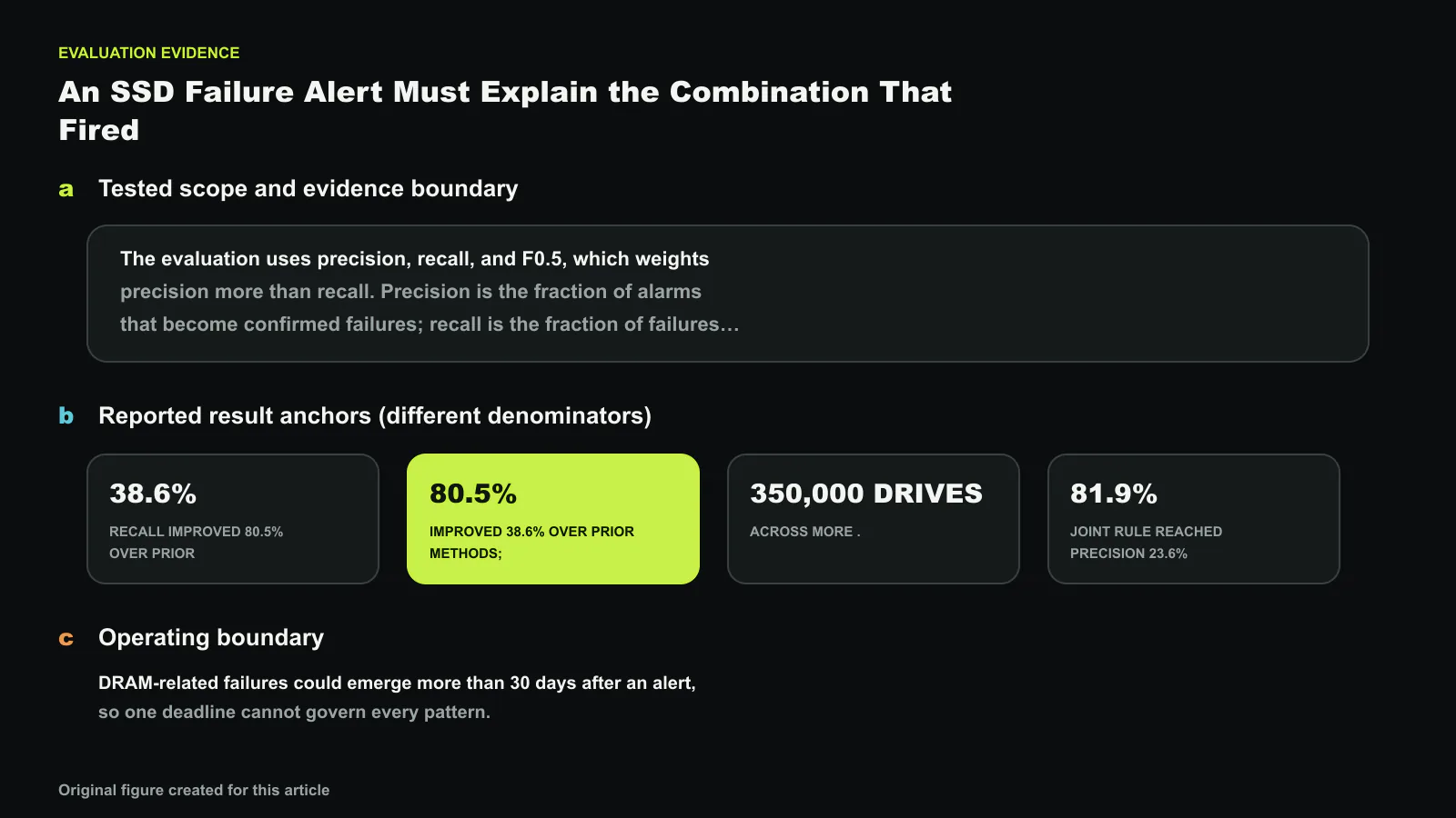
The evaluation uses precision, recall, and F0.5, which weights precision more than recall. Precision is the fraction of alarms that become confirmed failures; recall is the fraction of failures caught. At datacenter scale, even a low false-alarm rate applied to hundreds of thousands of healthy drives can create hundreds of migrations and replacements.
On real Tencent telemetry, the strong decisions raised average precision 38.6% over the evaluated prior approaches; the corresponding recall gain was 80.5%. One uncorrectable-error joint rule reached 81.9% precision and 23.6% recall. A random forest comparison reported 55.4% precision, while the MVTRF temporal-feature baseline reached 68.1% precision and 19.6% recall with F0.5 of 0.46.
These values describe different operating points, not a universal ranking of model families. Thresholds, observation windows, failure labels, drive models, and replacement policies affect both metrics. The Alibaba SMART dataset contained different attributes and served as a generalization check, but production deployment evidence came from Tencent’s fleet.
Ablation separated the mechanisms. Relative to the comparison path, boundary-preserving downsampling with a forest raised precision 21.7%, while recall rose 49.3%. Adding joint-key extraction improved them by another 20.4% and 25.5% in the cited analysis. The combined method produced the highest reported values.
Deployment needs lead time and an action for every rule
Strong decisions ran in Tencent datacenters for more than one year across over 350,000 SSDs. Alerts entered an operational process that could migrate service or replace a drive. For the uncorrectable-error decision, 51% of alarmed drives were reported failed within one week. DRAM-related failures could emerge more than 30 days after an alert, so one deadline cannot govern every pattern.
Lead-time distribution matters as much as recall. An alert arriving minutes before device loss may be accurate but unusable for migration. An alert months early ties up spare capacity and may replace a drive that would have served safely. Each joint decision should therefore carry its precision, expected failure-time distribution, affected model and firmware, and recommended action.
The rules also support causal investigation without proving causality. NandUECC thresholds identify observed uncorrectable errors; they do not establish whether NAND wear, read disturb, firmware, or workload initiated the chain. DRAM and capacitor signals can guide teardown and firmware analysis. Manufacturer feedback and hardware inspection are needed before changing a product design.
Weak decisions covered PCIe errors, bad blocks, and end-to-end errors. Their precision below 50% made them unsuitable as direct failure alarms, yet identified populations had higher subsequent failure rates than ordinary healthy drives. A lower-cost action such as increased monitoring, workload reduction, or scheduled maintenance can use those signals.
Fleet drift can invalidate a readable rule
Interpretability does not make a threshold permanent. SSD controller firmware, NAND generation, overprovisioning, telemetry definitions, workload mix, and fleet age change. A rule learned on one model can fire too often or miss a new failure mode on another. The production system needs rule versioning by model and firmware and ongoing calibration against confirmed outcomes.
Daily telemetry also creates temporal ambiguity. A delta depends on collection interval and missing samples. Clock drift, counter reset after power cycle, saturation, and vendor-specific units can mimic a failure pattern. Input validation should run before decision evaluation, with a distinct alert for unreliable telemetry.
Deployment monitoring should report alarm count, precision with delayed labels, recall, lead-time quantiles, migrations, replacements, service incidents prevented, and drives returned with no fault found. A fleet-level cost model can assign different prices to false positives and missed failures, then choose which strong and weak decisions trigger which action.
The method’s value is not that three rules replace machine learning. Random forests discover interactions in a high-dimensional fleet; joint mining compresses the useful routes into an operational interface. Retraining can change the rules, while operators retain the ability to audit why one drive was selected.
The actionable unit is an attribute combination plus time
FailureMiner shows why feature importance is too coarse for storage operations. “NAND errors matter” does not specify how many, how quickly they changed, what other condition must hold, or when failure tends to follow. A joint decision supplies thresholds and conjunction; deployment statistics supply precision and lead time.
The reported 38.6% precision and 80.5% recall improvements, one-year run, and 350,000-drive coverage establish practical promise. The result remains tied to the evaluated labels and fleets, and the low recall of some high-precision rules means it is not a complete failure shield. Buyers should ask how rules transfer across drive models, how outcomes are confirmed, and what happens to alarms that never become reported failures.
The strongest deployment uses a ladder of actions. High-precision rules with short lead time can trigger immediate migration. Longer-lead rules can schedule replacement. Weak decisions can raise sampling frequency. In that structure, model interpretation becomes resource allocation rather than a dashboard explanation.
Source and copyright notice
This article is an editorial analysis by Silicon & Systems. It restates the method, measurements, deployment evidence, and limits in our own words. No source sentence, table, or figure is reproduced; the figure was created for this article. The paper is available from the USENIX FAST 2026 presentation page. Copyright remains with the authors, 2026.