A congestion-control algorithm can win every standard benchmark and still fail in production. The problem may not be the implementation or the topology. It may be that the test workload produced the right flow sizes but the wrong sequence of pressure on the control loop.
A study from Carnegie Mellon University and Meta argues that burstiness should be treated as a coverage space rather than a traffic label[1]. It surveys datacenter-network evaluations, compares their synthetic workloads with 1-millisecond production measurements from Meta’s Millisampler, and organizes bursts along four dimensions: intensity, duration, sender synchronicity, and inter-arrival time. DCTCP is the case study used to show that different regions of those dimensions create different controller behavior.
The most useful result is methodological. A flow-size cumulative distribution function (CDF) says how many bytes a sampled flow contains. It does not say whether many senders align, how long offered load exceeds drain rate, or whether the next burst arrives before the controller recovers. Adding one incast pattern helps, but one manually selected point still cannot demonstrate behavior across the operating range.
A production burst has memory
The paper defines a burst at a network element as an interval in which arrivals exceed the element’s drain capability and utilization crosses a threshold. For its analysis, an interval above 50% utilization is considered bursty, consistent with the production-measurement method it adopts. The exact threshold is less important than using the same definition across production and simulation.
The production reference is Millisampler data collected at hosts across Meta’s fleet at 1-millisecond granularity. The authors focus on the Top-of-Rack (ToR) downlink to a receiver because incast converges there. They compare high-utilization sequences with simulated traffic on a 128-host fat tree using DCTCP.
Their temporal-clustering metric is an r-value derived from a two-state Markov model. An r-value of one means that the probability of a burst in the next interval does not depend on whether the current interval is bursty. Larger values indicate that high-utilization intervals cluster. Ten sampled production hosts have a mean r-value of about 36. Simulated burst-aware workloads have a mean near 7.3.
This difference is not simply “more traffic” in production. Production bursts are relatively rare, but once one starts, a bursty interval is more likely to be followed by another. Several simulated workloads create bursts more frequently but make them probabilistically shorter. Both traces can have bursts, yet they expose a reactive controller to different histories.
That history changes the controller state. DCTCP updates its congestion estimate and sending window over round trips. A burst arriving after a quiet recovery period meets a different window and queue than one arriving while the previous reaction is still settling. An evaluation that discards ordering can preserve a flow-size histogram while erasing the cause of a failure mode.
Most workload recipes specify demand, not controller stress
The authors examine six years of burst-relevant work spanning OSDI, HotNets, IMC, EuroSys, NSDI, CoNEXT, and SIGCOMM. They group evaluated workloads into four categories.
The first category samples an empirical flow-size CDF, commonly with Poisson arrivals and random endpoints. It leaves burst creation to chance. This recipe accounts for 45% of the surveyed papers. It can reproduce an average offered load and the distribution of object sizes, but it does not intentionally cross a congestion controller’s boundaries.
The second category adds a fixed incast pattern to background traffic. It accounts for 17.5%. The test now includes a synchronized many-to-one event, yet sender count, flow size, and query rate often remain at one selected point. The result demonstrates behavior at that point only.
The third category varies incast parameters and also accounts for 17.5%. It is the most expressive common method, but an arbitrary sweep has no guarantee of covering all controller regimes. Varying the number of senders while leaving burst duration and recurrence coupled may test the same behavior repeatedly.
The remaining 20% use fully synthetic workloads. These are valuable for microbenchmarks and targeted stress, especially when no public production trace exists. Their weakness is not artificiality by itself. It is the absence of an explicit mapping from synthetic parameters to the state transitions the algorithm is supposed to handle.
This taxonomy changes how benchmark quality should be judged. Realistic flow sizes are useful, but realism is not one scalar. A workload can match a CDF and miss temporal clustering. It can match average utilization and miss sender synchronization. It can match one incast size and miss the recurrence interval that creates standing congestion.
Four dimensions expose four kinds of boundary
Intensity is the amount of data injected when a burst begins. In the DCTCP case, the paper relates initial intensity to the number of incast flows and their initial congestion windows. Two relevant boundaries are the ECN marking threshold K and the available queue buffer B. Below K, the queue may remain in a healthy region. Above K, marking begins. If aggregate injection exceeds B, loss is unavoidable under the modeled conditions.
Duration is how long the burst persists. A burst shorter than one round-trip time can finish before senders receive useful feedback. A burst longer than a round trip but shorter than DCTCP convergence occupies a transient regime. A burst longer than convergence gives the controller time to settle while the event continues. The same peak rate can therefore produce different outcomes depending on how long it lasts.
Synchronicity describes the phase alignment of senders. Perfectly aligned senders can fill the bottleneck queue before any feedback returns. Marking then resembles a coarse binary event rather than a gradual proportional signal. Staggered senders let earlier congestion signals affect later arrivals, but low synchronization can also create fairness differences because individual flows enter different phases of their window cycle.
Inter-arrival time determines which controller state the next burst encounters. If the gap is long enough, the queue drains and the congestion estimate relaxes. If another burst arrives during recovery, it inherits a reduced or oscillating window, queued packets, and recent marking history. Repeated bursts can therefore create persistent behavior that no isolated-incast experiment reveals.
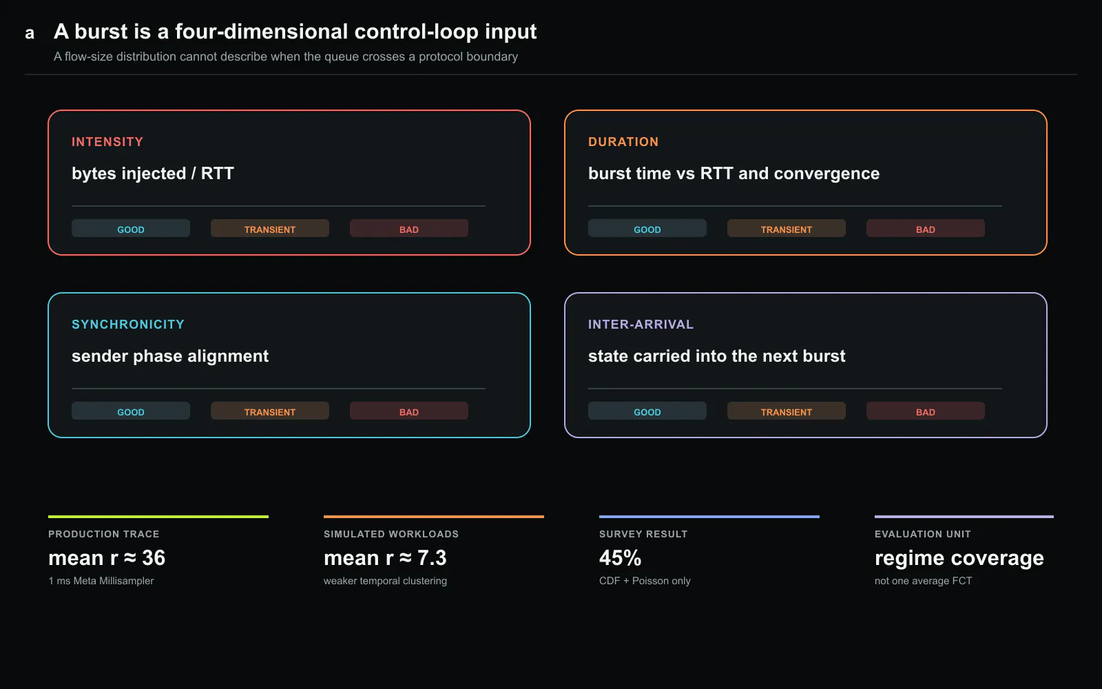
The dimensions also interact. High intensity can lengthen drain time. Synchronization changes effective intensity at the queue. Duration determines whether the controller reaches steady state. Inter-arrival time decides whether that state carries into the next event. A complete Cartesian sweep may be too expensive, but selecting parameters independently without considering these interactions can omit the most difficult corners.
DCTCP is evidence for the method, not a universal map
The paper uses DCTCP because its ECN threshold, window reaction, and convergence process make the boundaries explainable. The resulting regimes should not be copied directly to every congestion-control algorithm. An INT-based protocol that obtains detailed in-network feedback and chooses a rate within one round trip may collapse much of the duration axis. A delay-based controller reacts to a different signal. A receiver-driven design may define synchronization and recovery differently.
This limitation strengthens the methodological point. Every controller class needs its own behavior map. The workload generator should then cover the map, and a comparator should report where two algorithms differ. A benchmark that applies identical parameter values to all algorithms can still be unfair if those values cross a boundary for one algorithm but remain in one regime for another.
The DCTCP analysis is also a motivating case, not a complete empirical validation of the proposed stack. The paper does not provide a finished public generator that guarantees all four-dimensional coverage for every controller. It outlines three components: behavior-regime analysis, a burst generator, and a regime-aware comparator. A buyer should read this as an evaluation agenda with supporting evidence, not as a drop-in certification suite.
AI collectives make the missing dimensions more expensive
Traditional incast appears in partition-and-aggregate services, storage, and databases. AI training adds repeated collectives whose communication phases are aligned by computation barriers. A single delayed flow can hold the next iteration, leaving many accelerators idle. The economic denominator is therefore not only mean flow-completion time. It is collective completion and preserved accelerator work.
Collectives also create structure that random endpoint selection removes. AllReduce, All-to-All, broadcast, and parameter exchange have different fan-in, fan-out, path reuse, and recurrence. Expert parallelism can create destination skew. Pipeline stages can align several groups. Gradient synchronization repeats at a cadence tied to compute. A fabric test should preserve these structures while independently varying the burst dimensions.
RDMA changes the visible failure mode but not the need for burst coverage. A lossless configuration can avoid drops while queues and pause propagation raise latency. Packet spraying may distribute sustained load yet create reordering or expose short flows to a slow path. A controller can maintain high link utilization while one rail repeatedly becomes the straggler. Average throughput can hide the application penalty.
For training, report the distribution of collective completion time, iteration time, exposed communication, queue occupancy, ECN marking, pause duration, reordering, and fairness between simultaneous jobs. Then locate the burst coordinates of each result. Without the coordinates, another lab cannot determine whether it tested the same controller state.
Build a test matrix around boundaries
A practical test does not need to sample every numerical combination. It needs to cross each known boundary with margin. For intensity, test below marking, around the marking threshold, between marking and available buffer, and beyond the loss or pause region. Preserve offered bytes while changing sender count and per-sender window to separate aggregate intensity from synchronization.
For duration, hold peak intensity constant and test an event shorter than the round trip, one spanning several feedback cycles, and one longer than measured convergence. Record the controller state before, during, and after the event. A single completion-time number cannot show whether recovery continues after the burst ends.
For synchronization, vary sender start-time jitter from near zero to a value that spreads arrivals across multiple feedback intervals. Keep total bytes and destinations fixed. This reveals whether a result comes from lower instantaneous pressure or from a better control response.
For recurrence, first measure recovery time. Then schedule the next burst well after recovery, near the recovery boundary, and before recovery. Include non-periodic gaps because a perfectly periodic workload can synchronize with controller sampling or timers. The difficult case may occur when recurrence drifts through those phases.
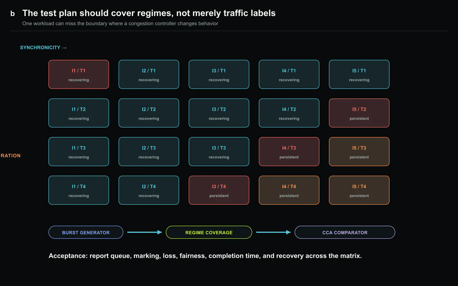
The matrix should include interactions selected by mechanism. Cross high intensity with short duration to test feedback latency. Cross moderate intensity with tight recurrence to test accumulation. Cross synchronization with large buffer to see whether avoiding loss merely converts the problem into tail latency. Cross recurrence with competing background jobs to test fairness and state carryover.
Production traces need privacy-preserving structure, not raw payloads
The study uses aggregated link-utilization samples rather than application payloads. That separation is operationally important. A benchmark does not need customer bytes to preserve temporal clustering. It needs a trace or generative model that retains when and where offered load concentrates, with sufficient metadata to map the result to topology and control-loop timescales.
One release method is to publish transition statistics and bounded multidimensional summaries rather than raw host identities. Another is a calibrated generator that reproduces run lengths, recurrence distributions, spatial fan-in, and load while removing service labels. Validation should compare generated and production traces across several statistics, not only the r-value used in this paper.
The statistics must be computed at relevant resolutions. A 100-millisecond sample can average away a microsecond-scale queue event. A very fine sample can create sparse noise that obscures application cadence. Report results across several windows and relate each to link serialization time, round-trip time, switch feedback interval, and collective phase length.
Production changes also require versioning. A workload calibrated before a new accelerator generation, transport, or placement policy may no longer represent current traffic. Store the capture interval, fleet segment, topology class, link rate, and preprocessing rules. A “production-like” label without those fields is not reproducible.
What this paper does not establish
The comparison uses selected production hosts and simulated workloads, not an exhaustive census of every Meta service or fabric. The mean r-values demonstrate a substantial fidelity gap for the studied traces and recipes. They do not define one universal target for all datacenters.
The burst threshold and Markov summary compress a complex time series. Two traces can share an r-value while differing in burst length distribution, intensity, or spatial correlation. The four-dimensional framework is intended to restore some of that missing structure, but its parameters and boundaries still need measurement for each environment.
DCTCP’s regimes are analytically motivated and illustrated, while the full behavior of modern production controllers may include hardware pacing, multiple feedback signals, priority flow control, retransmission, adaptive routing, and application scheduling. Those mechanisms can add state and timescales not represented in a one-controller case study.
Lastly, broad coverage does not guarantee operational safety. A test can discover a bad region, but the production system still needs admission control, telemetry, fallback, and rollout policy to avoid or contain it. Evaluation identifies the boundary; system design decides what happens near it.
The purchasing claim should be a coverage claim
When a switch, NIC, or congestion-control feature claims lower tail latency, ask which burst regions were tested. Request sender count, per-flow size, duration, start-time jitter, recurrence, background load, buffer configuration, path count, feedback interval, and controller parameters. Ask whether the workload was calibrated against production temporal statistics.
Compare algorithms by regime rather than one overall average. One controller may excel under sustained synchronized load while another recovers faster from short recurring events. The choice depends on the collective mix and the cost of a straggler. A weighted aggregate is meaningful only after the weights reflect the intended deployment.
The enduring insight is simple: traffic has order, and reactive control has memory. A CDF discards both. The four-dimensional framework restores a testable relationship between a burst and a controller’s state. For AI fabrics, that relationship should become part of every performance claim, because the expensive failure is not a busy link by itself. It is a synchronized workload reaching a controller state the benchmark never exercised.
Source and copyright notice
This article is an independent editorial digest by Silicon & Systems. It explains the paper’s survey, production-trace comparison, DCTCP case study, and limitations in original language. No source sentences, tables, or figures are reproduced. Both figures were created for this review with deterministic graphics. The full paper is available from the Carnegie Mellon Parallel Data Laboratory and is licensed under CC BY 4.0. Copyright (c) 2026 the authors.