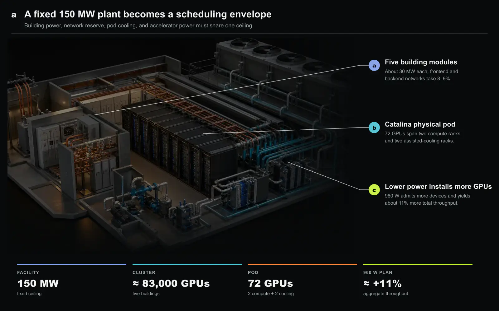
An AI datacenter does not buy GPUs one at a time. It buys a fixed electrical envelope years before the accelerators arrive, then converts that envelope into useful model tokens. A 2026 paper from Meta documents this conversion at unusual resolution: five roughly 30 MW buildings, about 83,000 GB200 GPUs and a 150 MW power ceiling[1]. The deployment is part of a larger 1 GW campus, but its most useful lesson fits inside one sentence. The GPU setting that maximizes a device benchmark does not maximize the work completed by the cluster.
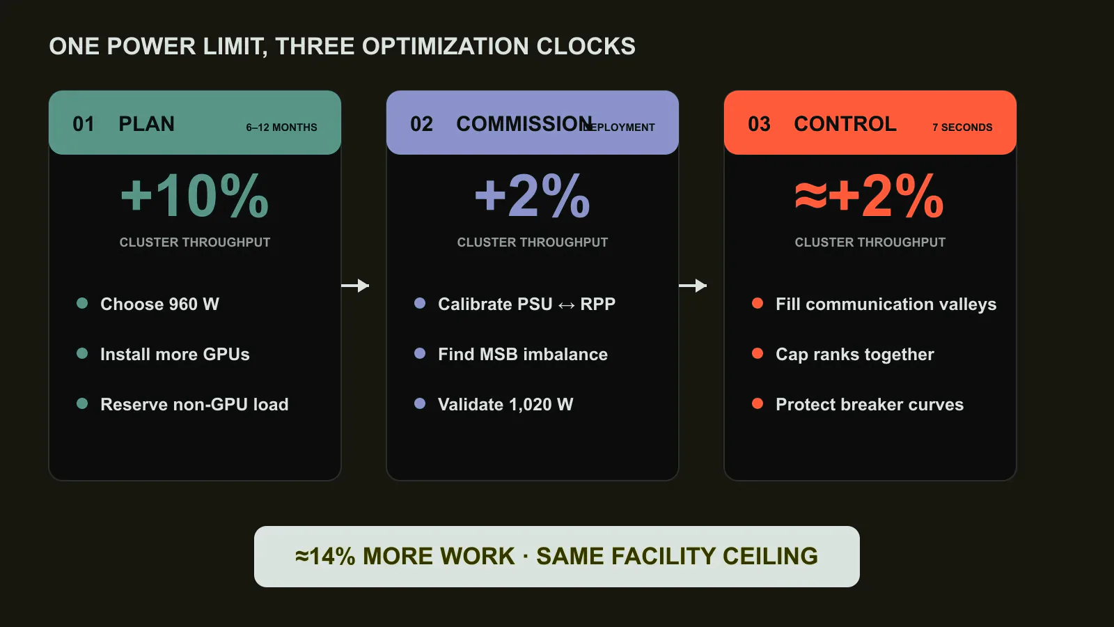
The authors follow the system from capacity planning through commissioning and live operation. Their result is not a new cooling loop or accelerator. It is a stack of decisions that jointly raises throughput by about 14% within the same facility limit. Specifically, Meta gains roughly 10% from fitting more GPUs at a lower initial power limit, about 2% after measured headroom permits a higher setting, and another 2% from a runtime controller. That ledger turns power from a procurement constraint into a schedulable cluster resource.
The 1,200 W GPU that loses to 960 W
GB200 can operate at a 1,200 W maximum GPU power setting, but Meta provisioned its deployment around 960 W. The apparent sacrifice is small at the device and large at the building. Reducing the setting from 1,200 W to 1,000 W cuts measured per-GPU performance by about 5% while reducing the power allowance by 16.7%. At 900 W, the respective changes are about 12% and 25%. Since a datacenter admits more accelerators when each one claims less of the electrical budget, the cluster throughput curve peaks below the device curve.
The paper normalizes this calculation against a 700 W H100 fleet under the same 150 MW ceiling. A 1,200 W GB200 plan fits about 74,000 GPUs and produces 1.7× the aggregate throughput of the H100 reference. At 960 W, the plan fits roughly 86,000 GPUs and reaches 1.9×. Thus, the lower setting yields about 11% more cluster work than the nominal maximum even though every individual GPU runs more slowly. Network radix and deployment details reduce the realized count to approximately 83,000, but do not change the decision.
This calculation must include everything that is not a GPU. The backend and frontend networks consume 8% to 9% of the entire 150 MW allocation. A Catalina compute pod combines two racks containing 72 GB200 GPUs in one NVLink domain with two air-assisted liquid-cooling racks, because the buildings lack facility chilled water. Every Grace CPU also carries two 400 Gb/s ConnectX-7 interfaces for the backend fabric and a separate 200 Gb/s frontend connection[2]. Power reserved for those paths cannot be sold twice.
Provisioning is a forecast, commissioning is an audit
Meta separates power management into three time scales. Planning begins 6 to 12 months before the next accelerator generation, when engineers have models rather than production measurements. Commissioning then checks those assumptions against rack and facility telemetry. Runtime control finally exploits short-lived headroom without placing breakers or jobs at risk.
The commissioning phase exposed why nameplate arithmetic is insufficient. Rack power-supply telemetry consistently reported more power than the upstream remote power panel (RPP) measured. Meta calibrated the former against the latter and found that a 70th-percentile aggregation represented the shared load better than a simple maximum. The discrepancy is not bookkeeping trivia. A conservative error multiplied by 83,000 GPUs strands megawatts that could have performed useful work.
Physical distribution also creates local limits inside a healthy building. Power flows from main switchboards (MSBs) through RPPs to racks, and the tightest element determines whether another watt is usable. The deployment showed that 13% of MSBs had less than 50 kW of remaining capacity. Average MSB headroom was around 160 kW, equivalent to about 100 W per GPU beneath that board, while RPPs retained more than twice as much on a per-GPU basis. Consequently, 5% to 10% of provisioned capacity could remain stranded behind imbalance even when the campus total looked comfortable.
Measurements nevertheless justified a controlled increase in the GPU setting from 960 W to 1,020 W. That step recovered an expected 2% to 3% of performance without changing the number of installed accelerators. The sequence matters: the original lower limit bought physical density, and only the audit established where some of the reserved margin could safely return to computation.
Flatten the pulse, then dim the fleet
Large synchronous jobs do not draw steady power. Compute phases raise demand together, while communication phases lower it together. A cluster-wide transition can therefore create a sharp pulse even when average consumption stays below the limit. Breakers tolerate overloads for a short interval, but the paper reports operational curves of roughly 1.2× for 45 seconds or 2× for 30 seconds. A controller that reacts after a long averaging window is protecting the wrong time scale.
The consequence can extend beyond the building. The Llama 3 report observed changes of tens of megawatts when a 24,000-GPU job entered or left synchronized compute, and SemiAnalysis subsequently framed the same load shape as a grid-interface problem rather than only a datacenter power problem[5][6]. This does not make dummy work inherently efficient. It shows why the cost of smoothing must be compared with the electrical reserve that an unmanaged step would force upstream.
Meta deploys two complementary mechanisms. Power Smoother fills predictable communication valleys with tensor-core instructions that use registers rather than HBM or L2. The extra operations do no application work, but they prevent the electrical system from repeatedly falling and surging. An adaptive backoff keeps the mechanism within the available budget, and the reported application cost stays below 3%. The trade is deliberate: a small amount of wasted arithmetic reduces a physical transient that could force a much larger safety margin.
Dimmer handles the remaining peaks. When device readings exceed 97% of an applicable limit, it gradually adjusts GPU caps using a seven-second average. Coordination is essential. An uncoordinated cap would slow one worker, turn it into a distributed-training straggler and leave the other workers consuming power while waiting. Dimmer therefore works with job and scheduler context so that ranks sharing a workload are adjusted together. The controller contributes roughly another 2% of cluster throughput by making temporary headroom usable rather than permanently reserved.
What operators should copy
The transferable idea is not the precise 960 W value. That number belongs to one accelerator, workload mix, network and building. The transferable unit is the optimization boundary. If the objective is device performance, the answer is the highest stable accelerator setting. If the objective is completed cluster work under a facility ceiling, the answer must include GPU count, non-compute loads, electrical hierarchy, workload synchrony and recovery from local imbalance.
This boundary also changes the role of telemetry. Rack sensors, RPP meters and MSB limits describe different parts of the same resource graph. Treating any one stream as ground truth either risks overload or strands capacity. The paper’s 14% result comes from closing the loop across time: forecast conservatively, measure at deployment, then spend verified headroom with coordinated controls.
There are limits to the comparison. The aggregate throughput estimates use Meta’s workload characterization and a specific generation transition. A service dominated by latency-sensitive inference may value the last watts differently from a dense training fleet. Power Smoother also exchanges energy for a flatter profile, so its merit depends on how the utility, cooling system and breaker hierarchy price transients. Even with those qualifications, the central accounting remains robust. At 100 MW scale, power is no longer an attribute of the cluster. Power is the cluster.
A commissioning model for the next 100 MW
The paper is most useful when translated into a commissioning model rather than a list of settings. Start with four ledgers that remain separate until the final capacity decision. The first records contractual facility power at each building. The second subtracts electrical conversion, cooling, networking and control loads. The third maps the remaining power through MSBs, RPPs and rack feeds. The fourth converts the deliverable rack envelope into workload throughput at several accelerator caps. Combining these ledgers too early hides the location of the limiting constraint.
Consider the 150 MW example. If networking consumes 8% to 9%, it claims 12 to 13.5 MW before the first training step. Cooling and conversion losses consume additional capacity even though they do not appear in a GPU telemetry stream. The remaining budget cannot be divided by 960 W, because a GB200 compute module includes CPUs, memory, local fabric and power delivery. It also cannot be divided evenly across buildings when one MSB is nearly full and another has substantial headroom. The correct divisor is therefore the measured, topology-aware power of a deployable pod.
This distinction explains why a campus can show two apparently contradictory facts: unused power at the utility meter and no safe location for another rack. The utility meter describes an aggregate. The constrained MSB describes an address. Capacity becomes useful only when it has both quantity and location. A commissioning report should consequently publish a distribution of headroom by electrical node, not only a campus percentage. The lower tail of that distribution determines how many planned racks can actually be energized.
Telemetry accuracy needs the same hierarchy. Device-reported power is valuable for rapid control, while RPP and MSB meters are better suited to protection and reconciliation. Their sampling windows, calibration errors and physical boundaries differ. A peak in a subsecond device trace may disappear in a facility average, while a systematic rack bias can accumulate into several megawatts in the plan. Operators should preserve raw measurements, align timestamps and fit an explicit transfer model between layers. Replacing the model with a single correction factor would assume that the error is constant across workload, temperature and utilization.
The 70th-percentile aggregation reported by Meta should not be copied as a universal constant. It is evidence that a carefully selected statistic can match the shared electrical boundary better than summing independent maxima. Another site may need a different percentile because its workload mix, power supplies and meter windows differ. The validation rule is straightforward: choose the statistic on historical commissioning data, then test it on separate high-load periods. A value that only fits the calibration run is not usable headroom.
Separate energy, power and ramp rate
Three quantities are easily collapsed into one dashboard. Energy determines the bill over an interval. Power determines whether a feeder or cooling plant can sustain the load. Ramp rate determines whether the electrical system and grid interface can follow a synchronized transition. Power Smoother may increase energy while lowering ramp rate, whereas Dimmer reduces a peak by temporarily lowering compute throughput. Calling either mechanism simply “power optimization” obscures the different cost it pays.
The distinction also determines the experiment. To evaluate a cap, measure completed model work, joules and wall-clock time. To evaluate smoothing, measure the distribution of positive and negative ramps at the relevant electrical boundary. To evaluate a protection controller, test the tail of response latency and the maximum overshoot, not only the mean. A controller that looks efficient over an hour can still trip a breaker during a short synchronized phase transition.
Power Smoother is rational only when the value of a flatter load exceeds its added energy and possible application interference. That value can come from a smaller reserved margin, a less severe utility ramp constraint or more stable cooling operation. The comparison should be made at the boundary that actually imposes the limit. Smoothing a GPU trace that does not materially change the MSB or campus waveform produces cost without facility benefit.
Dimmer poses a different validation problem. Distributed jobs amplify unequal throttling because every rank waits at a barrier. A nominal 2% cap on one worker can cost more than 2% at the job level if it repeatedly becomes the slowest rank. The unit of actuation must therefore follow the synchronization domain. For tensor-parallel or pipeline-parallel jobs, that domain may be a subset of the allocation; for a tightly synchronized data-parallel job, it may span the entire job. Scheduler metadata is not an optional convenience here. It defines which devices must move together.
Treat headroom as inventory with an expiration time
Verified headroom is not permanent capacity. Ambient temperature changes cooling demand, firmware changes device behavior, model architectures change the compute-to-communication ratio, and a new network topology changes non-GPU power. Every headroom estimate should carry the measurements that justify it, the operating conditions in which it is valid and an expiration rule. A cap increase approved for one workload generation should be revalidated before it becomes the default for another.
This turns commissioning into a continuing accounting process. A useful control table would record the facility node, safe continuous limit, short-duration overload curve, calibrated measurement uncertainty, currently admitted load and remaining margin. The scheduler can then distinguish three kinds of capacity: continuously deliverable power, temporary burst allowance and unverified theoretical slack. Only the first should support long-running admission decisions. The second can support coordinated runtime boosts, and the third remains unavailable until measurement converts it into evidence.
Failure policy belongs in the same table. If a meter stream disappears, the controller should fall back to a conservative cap rather than assume the last observed margin persists. If a power command reaches only part of a distributed job, the scheduler should either complete the coordinated change or roll it back. If an MSB approaches its limit while the campus total remains safe, placement should move future work away from that branch. These cases show why facility control cannot be bolted onto a device management service after deployment.
Finally, report uncertainty alongside the throughput gain. The 14% ledger contains gains from different evidence levels: a planning comparison, a commissioning adjustment and runtime measurements. Future deployments should preserve that separation. A procurement model may estimate how many devices fit; commissioning proves how many can be energized; production telemetry shows how much accepted work they complete. Keeping those claims distinct makes the result auditable and prevents a modeled maximum from being presented as sustained service capacity.
The practical lesson is a design sequence. Reserve the facility boundary, model several device caps, place non-compute loads explicitly, and design the electrical topology so that capacity is reachable. Then calibrate every telemetry layer, validate a safe continuous setting and expose job synchronization domains to the controller. Only after those steps should an operator spend transient headroom. In this sequence, software does not evade the physical limit. It makes more of the purchased limit deliverable.
Throughput per deliverable megawatt is the real accelerator metric
The paper makes accelerator power a software-visible resource. Nameplate wattage is needed to protect wiring and cooling, but it is a poor predictor of useful facility output. A lower cap can sometimes improve cluster throughput per megawatt because frequency falls less than power, while a badly chosen cap can lengthen a synchronized job enough to erase the saving. The relevant curve is accepted tokens or training steps per deliverable megawatt at each cap, including the tail behavior of the slowest devices.
This changes procurement comparisons. Two accelerators with different thermal design power cannot be ranked by FLOPS per chip or watts per rack alone. The datacenter must include power-conversion losses, cooling, workload utilization, communication stalls, and the amount of headroom reserved for model error and transients. A nominally more efficient device can yield less campus output if its power excursions force a larger margin or if software cannot keep it in the efficient region.
The operating loop should therefore retain a power forecast error budget. Before deployment, planners need a confidence range rather than one peak estimate. After commissioning, rack and workload telemetry should update that range. At runtime, power caps and placement can spend the remaining margin where it creates the most useful work. The 150 MW system is significant because these are not separate facility and computing decisions. Provisioning sets the safe envelope, measurement identifies unused margin, and scheduling converts that margin into model progress. In an electricity-constrained market, that loop can create more sellable AI capacity than another percentage point of chip-level efficiency that never reaches the building boundary.
The electrical envelope must reach the scheduler
A cluster scheduler usually sees GPUs, memory, topology, and job priority. A power-limited scheduler also needs the capacity available at each time horizon. Utility delivery, substation and busway limits, rack power, cooling conditions, and short transient headroom are different constraints. Collapsing them into one site megawatt value either strands equipment or permits a local limit to trip before the global limit is reached.
The control hierarchy should match those horizons. Fast device controls can absorb millisecond and second excursions. Rack or row controls can rebalance minutes of sustained load. Job placement and admission can respond over longer intervals. A slower controller must not chase a transient that a lower layer already handled, and a fast controller must not conceal a persistent shortage until thermal or electrical margin is exhausted.
Workload information makes the hierarchy useful. Training steps often create synchronized power structure, while inference demand follows arrivals and batching. Checkpointing, data loading, and communication phases can lower or shift compute power. The scheduler can place jobs with complementary profiles, but only if power telemetry is aligned with job phase and the policy preserves performance and fairness.
Derating needs a performance denominator
Reducing a GPU from its maximum power can improve fleet throughput when it allows more devices to operate inside the same site limit. It can also lengthen a job enough to increase total energy or delay a synchronized training pipeline. The correct comparison is completed work per deliverable megawatt, with time and quality held to the service objective.
This denominator should be evaluated across the power curve rather than at two settings. Some workloads lose little performance over an initial reduction and then cross a sharp knee. Others are memory or communication bound and barely respond. A fleet controller can assign different limits by workload and phase, but the acceptance test must include tail step time, convergence or output quality, and any thermal effect on neighboring devices.
Derating also interacts with failures. Operating closer to a facility limit leaves less room when a cooling unit, power shelf, or link fails and work moves elsewhere. The reserve used for electrical resilience should be visible beside the compute reserve. Otherwise, a plan that looks efficient in steady state can shed more jobs during an ordinary maintenance event.
A 150 MW site is not 150 MW of sellable compute
Nameplate utility capacity loses margin through conversion, cooling, networking, storage, host CPUs, redundancy, and operational reserve before reaching accelerators. The usable amount also changes with weather, equipment availability, and the workload’s transient profile. Capacity sales should therefore specify a deliverable power envelope and the compute performance associated with it, not infer GPU count from a single arithmetic division.
Commissioning should verify the envelope from the bottom up. Exercise representative racks, rows, and failure scenarios; compare telemetry across utility, distribution, rack, and device meters; and reconcile losses. Then run synchronized workloads that reproduce expected pulses. A smooth synthetic load can validate wiring while missing the control problem that appears when thousands of accelerators change phase together.
We read the 83,000-GPU result as evidence that runtime power control is part of cluster architecture. Provisioning alone cannot guarantee useful capacity, and throttling alone cannot create it. Forecasting, commissioning, telemetry, scheduling, and device controls must share one model of the power path. The operational product is the amount of model work the site can complete continuously inside that verified envelope.
Source and attribution
This article is an editorial summary prepared for Silicon & Systems. It restates the cited paper in our own words. No text, tables or figures from the paper are reproduced; both figures were created for this article from reported results. The paper is available under the Creative Commons Attribution 4.0 International license. Copyright (c) 2026 the authors. The source paper and license are available through its arXiv record.