An edge sensor and an AI cluster can both claim better energy efficiency while measuring different work, accuracy, and system boundaries. MLPerf Power addresses that problem with one methodology spanning microwatts to megawatts, built by participants from more than twenty organizations[1].
The important message is that energy efficiency is not a device property until the completed work, quality target, measurement interval, and included infrastructure share one boundary. This review explains which comparisons the methodology makes defensible and where operators must still add cooling, idle power, or service-level behavior before using a result for procurement.
Define the boundary before comparing the number
The framework synchronizes useful-work and power measurement, specifies idle treatment and measurement equipment, and inherits MLPerf’s correctness thresholds. Sixty systems yielded 1,841 results that passed the reproducibility rules. Its central contribution is procedural: energy must be reported with the workload, scenario, quality target, and components included in the meter.
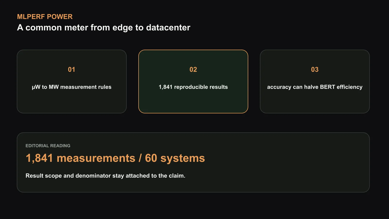
Results show why that discipline matters. In the reported BERT submissions, moving from 99% to 99.9% accuracy made inference about half as energy-efficient on average, although some systems resisted the loss. Diffusion image generation consumed 1,082× more energy per inference than the paper’s smallest compared workload. Data movement also grows into a first-order term at system scale and can be missed by device-only power readings.
Energy needs a matched unit of useful work
Power in watts is a rate, so it cannot rank systems without the amount and quality of completed work. Energy per inference integrates that rate over time, but it remains ambiguous when one submission uses a smaller model, lower accuracy, different batch, or a latency regime that the application cannot accept. MLPerf Power attaches the energy measurement to an existing benchmark workload and its quality rules.[1]
This coupling prevents a common optimization failure. Lowering precision, pruning, early exit, or reducing iterations can save energy by doing less of the requested task. Such changes are valid only when the output remains within the benchmark’s target. The BERT result shows that a stricter quality level can alter efficiency by roughly 2× on average, so accuracy belongs in the denominator rather than in a footnote.
Useful work also depends on scenario. An offline system maximizes throughput over a known batch, while a server must satisfy latency as requests arrive. A small device may process one sample at a time and spend much of its life idle. The same accelerator can occupy different energy operating points across those regimes.
Synchronizing power and work is the core measurement problem
A power meter produces samples over time while the benchmark counts completed queries. The run needs clear start and stop boundaries so setup, warm-up, and postprocessing are either consistently included or excluded. Clock mismatch between the load generator and meter can shift an energy window enough to matter for short tests.
MLPerf Power specifies measurement equipment, sampling, synchronization, and validity conditions across scales. A microwatt edge device and a megawatt-class installation cannot use the same physical instrument, but both must establish traceability and adequate resolution for the claimed result. Calibration, sensor placement, and uncertainty are therefore part of reproducibility.
Run duration matters. A short burst can exploit cold silicon, charged batteries, or temporary boost states. A sustained run exposes thermal limits, fan power, and stable clocks. Repetition reveals variability from scheduling, background services, and ambient conditions. The benchmark rules turn these details into an auditable procedure rather than trusting a dashboard average.
Idle energy belongs to some decisions and not others
An always-on endpoint may spend far more time waiting than inferring. A heavily loaded datacenter accelerator can amortize idle power across many requests. MLPerf scenarios and idle treatment help distinguish these cases, but readers still need the duty cycle of their deployment.
Energy per inference at peak throughput can understate the annual consumption of a lightly utilized server. Conversely, adding the full idle power of a shared host to one intermittent model can overstate its marginal cost. Capacity planning should evaluate both the benchmark’s standardized point and a utilization-weighted model for the intended service.
Batching exposes another trade-off. Larger batches often improve accelerator utilization and energy per item, but they add queueing latency and memory use. A server result must meet its latency constraint; an offline pipeline may choose a larger batch. Reporting only the most efficient point hides whether it is deployable.
The measured boundary can reverse a comparison
Device-only readings capture accelerator power but omit host CPUs, DRAM, network interfaces, storage, fans, power conversion, and cooling. These components can be small for a compute-heavy kernel and dominant for a distributed or movement-heavy workload. A system that reduces accelerator joules while increasing host preprocessing or communication may not reduce facility energy.
The correct boundary depends on the decision. Chip architects may need rail-level accelerator energy to isolate a design change. Buyers need server or rack power. Facility planners need power-usage effectiveness and cooling. MLPerf Power makes the selected boundary explicit so results at different levels are not silently combined.
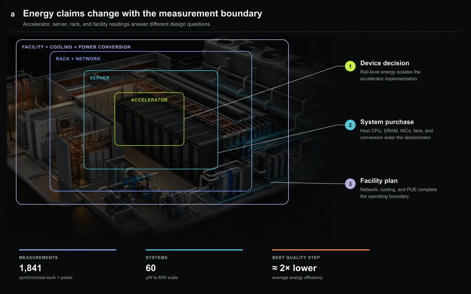
Data movement is particularly sensitive to boundary. A meter on the device sees HBM and compute but may miss network switches or storage that supply inputs. At cluster scale, collective communication and duplicated host work can consume energy not represented by an accelerator specification. The paper’s cross-scale framing makes this omission visible.
Accuracy is an energy control knob
The BERT 99% and 99.9% comparison is not merely a benchmark quirk. Higher quality can require a less aggressive quantization, a larger model, more calibration, or execution paths that reduce hardware utilization. The average efficiency roughly halved in the reported submissions, but the spread shows that some system and software combinations handled the stricter target better.
This suggests a better way to compare improvements. Plot energy against achieved quality and latency rather than selecting one point. A technique that saves 30% energy at unchanged accuracy is different from one that saves 30% while approaching the minimum acceptable threshold. Applications with asymmetric error costs may choose a point above the benchmark requirement.
Quality measurement itself has uncertainty and task dependence. A single scalar may not capture rare classes, safety constraints, or generated-output preferences. MLPerf provides a reproducible gate; deployments still need domain validation before converting benchmark efficiency into a product setting.
Workload choice changes energy by orders of magnitude
The 1,082× range between diffusion generation and the smallest compared inference illustrates why “AI inference energy” is not one category. Model size, number of iterative steps, data type, input dimensions, memory traffic, and quality target change the amount of work. Even within one task, preprocessing and postprocessing can move the system boundary.
A portfolio should therefore report energy by workload and service volume. Multiplying joules per inference by annual requests estimates operational energy, while peak power determines electrical provisioning. A low-volume expensive task can use less annual energy than a highly efficient task called billions of times.
The dataset of 1,841 results across 60 systems is valuable because it supports distributions and trade-offs rather than one winner. It can reveal which optimizations generalize across workloads, where accuracy costs appear, and how scale affects the share of noncompute energy. It should not be collapsed into a league table whose entries use different tasks.
Reproducibility requires configuration disclosure
A valid result needs hardware, firmware, software, model, precision, batch or scenario, quality, meter, sampling method, and power boundary. Accelerator clocks and power limits should be stated. For clusters, node count, network, host configuration, and cooling inclusion matter. Without these fields, another operator cannot reproduce either the work or the energy.
Software versions deserve the same attention as silicon. Kernel fusion, quantization, graph compilation, and request scheduling can change energy substantially. Comparing a tuned stack on one system with a default stack on another assigns software work to hardware. Benchmark rules reduce this risk, while transparent submission details let readers judge remaining asymmetry.
Uncertainty should be visible. Meter accuracy, sampling interval, run variability, and rounding can exceed a small claimed improvement. Repeated trials and confidence ranges prevent noise from becoming an efficiency record. Very large differences remain meaningful, but close results need disciplined statistics.
From benchmark result to facility decision
Buyers should begin with the workload, quality, and latency they actually need, then select matching submissions. They should translate benchmark energy into expected utilization, idle time, redundancy, and annual service volume. Peak system power determines rack density and electrical capacity, while energy determines operating cost and emissions under the chosen electricity mix.
Facility cooling and power conversion should be added consistently. A direct-liquid-cooled cluster may spend less fan energy but require pumps and facility equipment outside the server meter. Power usage effectiveness is a site property, not an accelerator property. Applying one PUE assumption to all candidates can be reasonable for an internal comparison if the cooling architecture remains the same.
The result should inform sensitivity analysis rather than a single purchase answer. Test how conclusions change with utilization, energy price, accuracy, latency, and model growth. A system with better current joules per inference may lose its advantage if the future workload exceeds memory and adds network traffic.
What architects can learn from the dataset
Separating device and system boundaries reveals whether compute, memory, host, or network dominates. If quality increases double energy, precision support and algorithm-hardware co-design are likely opportunities. If larger systems spend more outside the accelerator, interconnect and data placement deserve attention.
Longitudinal submissions can separate hardware gains from software gains when configurations are recorded. The same system with a new compiler shows software progress; the same stack on a new device approximates hardware progress. Neither comparison is perfect, but the standardized procedure creates a much stronger basis than vendor-selected power claims.
The benchmark can also expose rebound effects. A more efficient inference may lower cost enough that demand grows and total energy rises. MLPerf Power measures the unit cost; product and policy analysis must still multiply by usage.
Limits of one standardized framework
No finite suite covers every model, custom operator, latency target, or deployment. Submitted systems are selected and tuned by participants, so the dataset does not represent the average installed fleet. Results can age quickly as software and models change.
The framework is strongest as a measurement grammar. It requires work, quality, scenario, boundary, and energy to be stated together. A deployment should reproduce that grammar with its own traffic and facility conditions rather than treating the published table as a universal ranking.
Optimization claims should survive a boundary ladder
A useful internal review can measure the same workload at four nested boundaries: accelerator rails, complete server, rack including network, and facility allocation including cooling and conversion. The absolute energy rises at each step, but the change between a baseline and optimized system reveals where savings persist or migrate.
Suppose quantization cuts accelerator energy by 35% but adds host preprocessing and reduces batch flexibility. The device result may remain strong, the server improvement may be smaller, and the facility result may shrink again if the service needs more replicas to satisfy latency. Conversely, an interconnect optimization may barely move rail energy while substantially reducing rack energy and completion time.
The ladder also prevents inappropriate comparisons. A chip-team measurement can be valid for design analysis without being presented as facility energy. A buyer can request the server and rack levels relevant to procurement. Each level should use the same work, quality, and timing window so the difference is genuinely the added boundary.
Carbon and cost require time and location
Joules per inference can be converted into electricity cost only with workload volume and local tariffs. Carbon impact additionally depends on the time-varying generation mix and marginal electricity source. Two identical systems can have different emissions when operated in different regions or scheduled at different hours.
Carbon-aware scheduling may shift flexible offline inference to lower-emission periods, but interactive workloads cannot always wait. Moving work across regions adds network energy, latency, and data-governance constraints. Embodied emissions from manufacturing are another boundary and should not be inferred from operational power alone.
MLPerf Power supplies the reproducible operational unit needed for these calculations. It does not supply utilization, demand growth, electricity mix, or product lifetime. Keeping those layers separate allows the benchmark to remain technical evidence while business and environmental models state their own assumptions.
Procurement should retain absolute energy and power beside normalized efficiency. A system can deliver superior joules per inference yet draw more peak power because it completes far more work. That may be desirable, but it affects rack density and connection capacity. Conversely, a low-power device can have poor energy if it runs much longer.
Results also need an expiration policy. New model revisions, quality requirements, firmware, and compilers can move the operating point without changing the hardware name. Re-running a stable subset periodically shows whether the expected facility savings still exist and prevents an old record from pricing a new workload. An archived result should remain reproducible, but current buying guidance should identify the newest validated software and model generation rather than silently mixing submission dates. This version discipline matters when software gains are comparable to the hardware differences under consideration. It matters operationally.
What we take from it
MLPerf Power does not produce one universal winner. It makes the denominator auditable. Buyers should ask whether a result includes accelerators, host CPUs, networking, cooling, and idle periods, and whether quality targets match. Architects should use the same rules longitudinally so hardware, software, quantization, and scheduling improvements can be separated rather than collapsed into marketing efficiency.
The measurement boundary determines the buying decision
Power results become comparable only when the electrical and workload boundaries match. Accelerator-board power excludes host CPUs, memory, networking, storage, and cooling, while a rack or facility meter includes resources shared with other jobs. The workload boundary also matters because data loading, compilation, checkpointing, warmup, and idle gaps can move energy outside the measured interval. A lower device-level number can coexist with higher facility energy per completed result.
An evaluation should therefore publish synchronized timestamps for workload phases and each available meter. From those records, operators can calculate joules per completed training sample or SLO-valid inference, peak power for provisioning, and energy during nonproductive intervals. They should also report the measurement uncertainty and sampling rate because short power excursions can disappear in a coarse average. MLPerf’s enduring value is a common workload and disclosure structure. Procurement still requires mapping that structure onto the buyer’s own facility boundary and utilization pattern.
Source and attribution
This article is an independently written digest with two original figures. It reproduces no paper prose, chart, or table. The public preprint is available on arXiv; the authoritative proceedings version is © IEEE 2025.